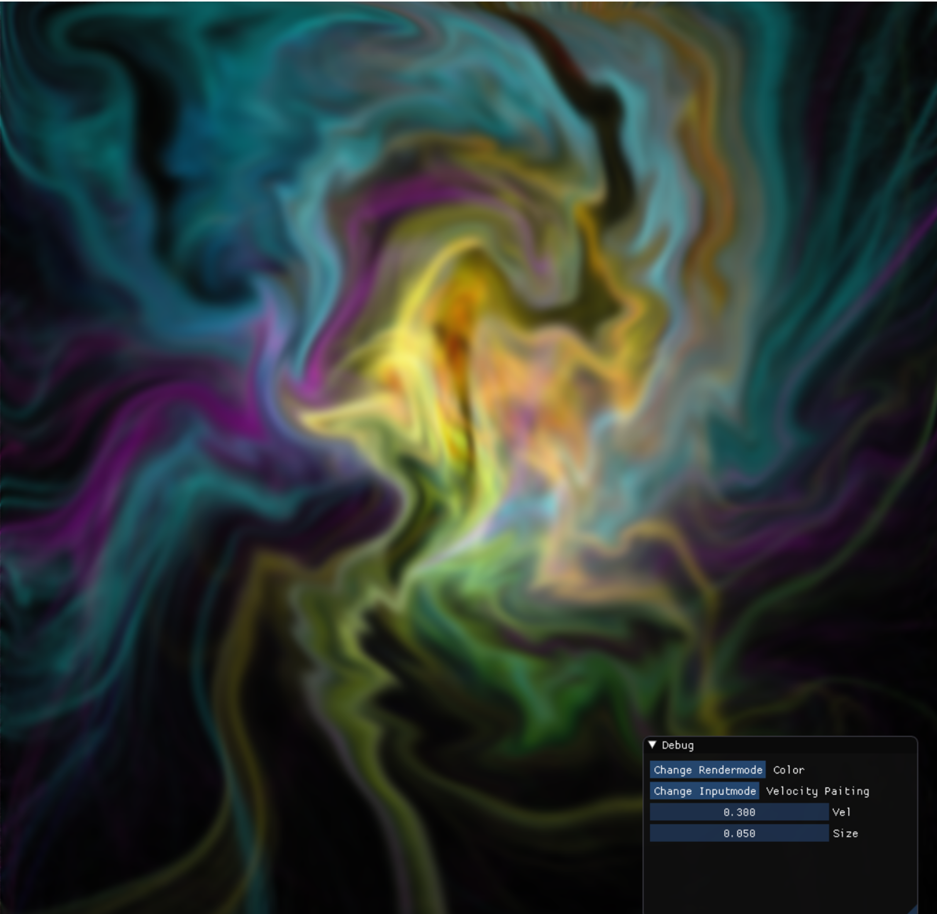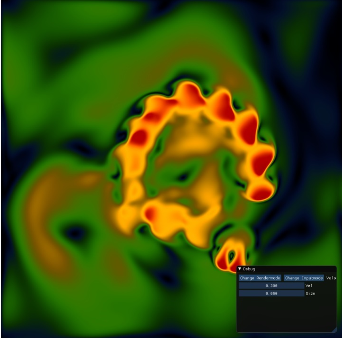
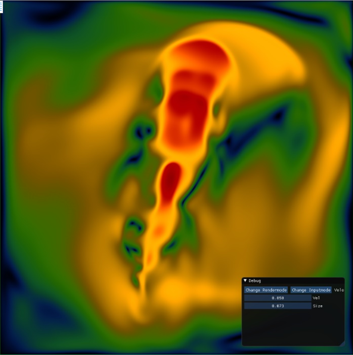
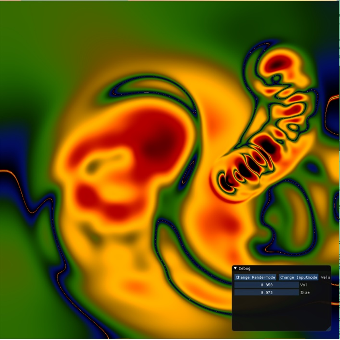
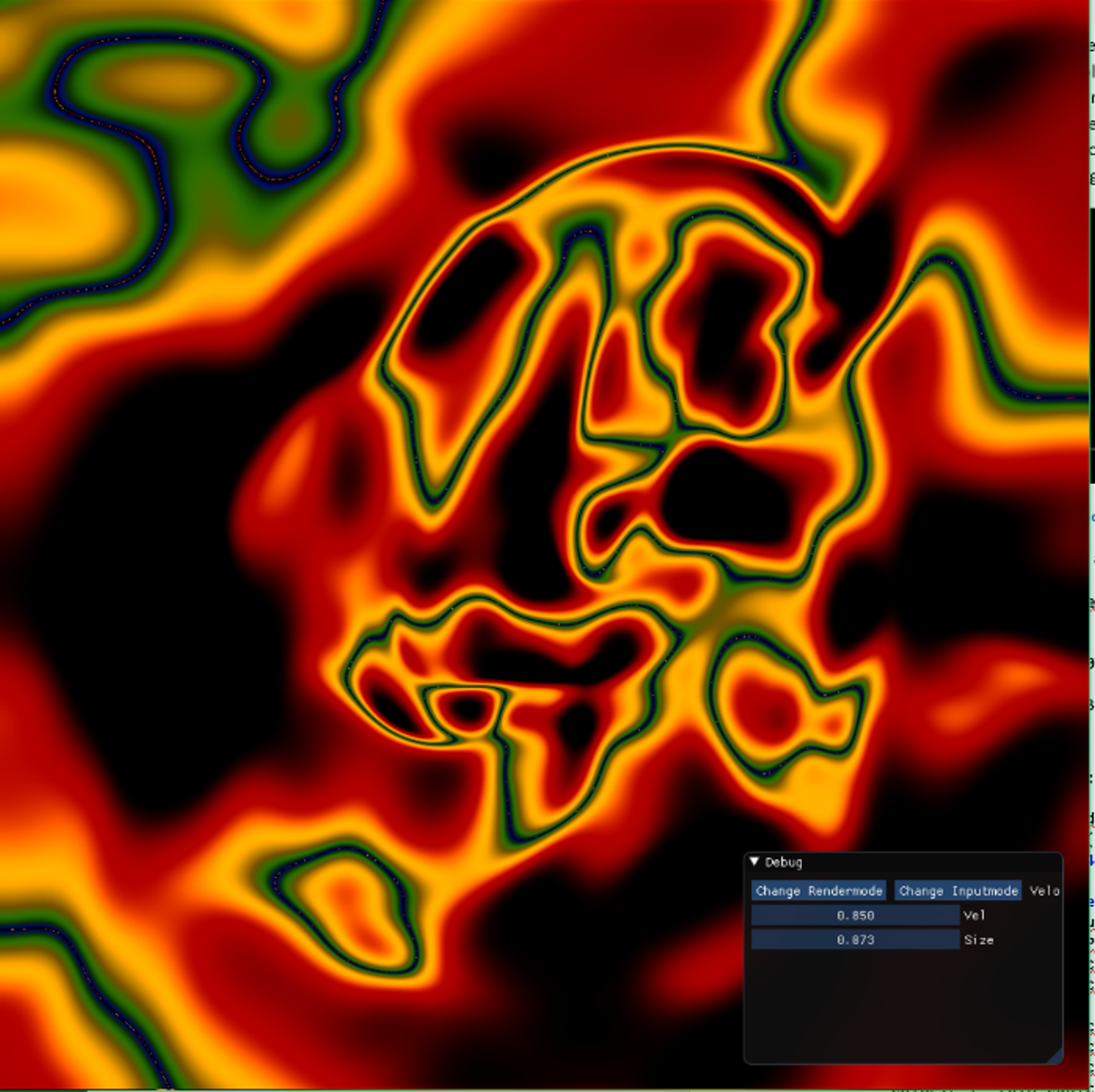
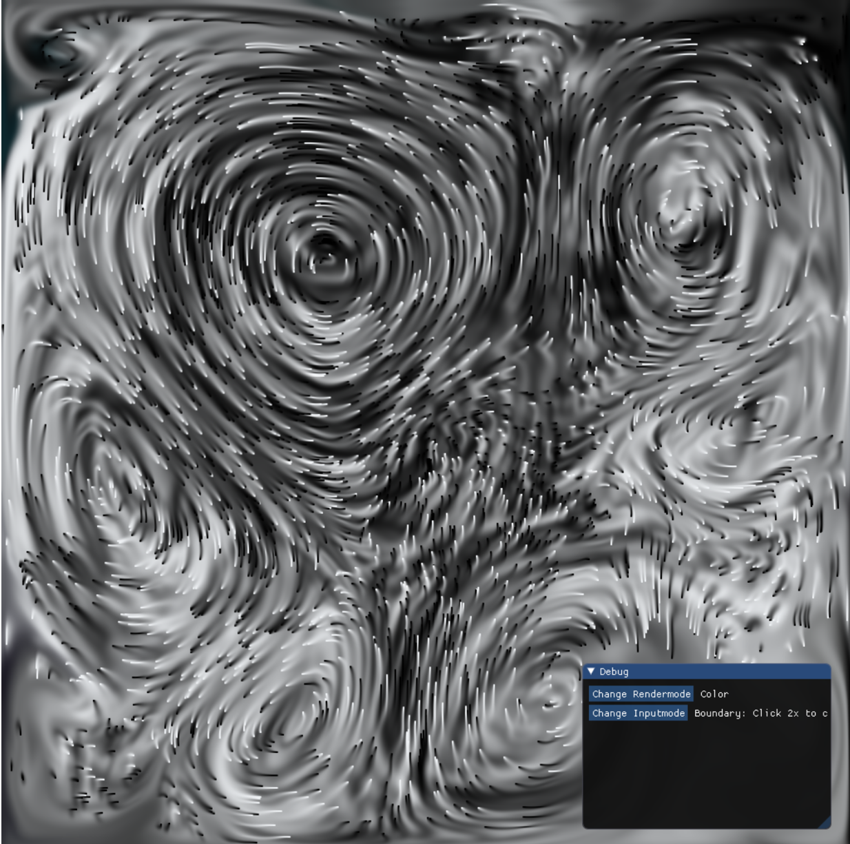
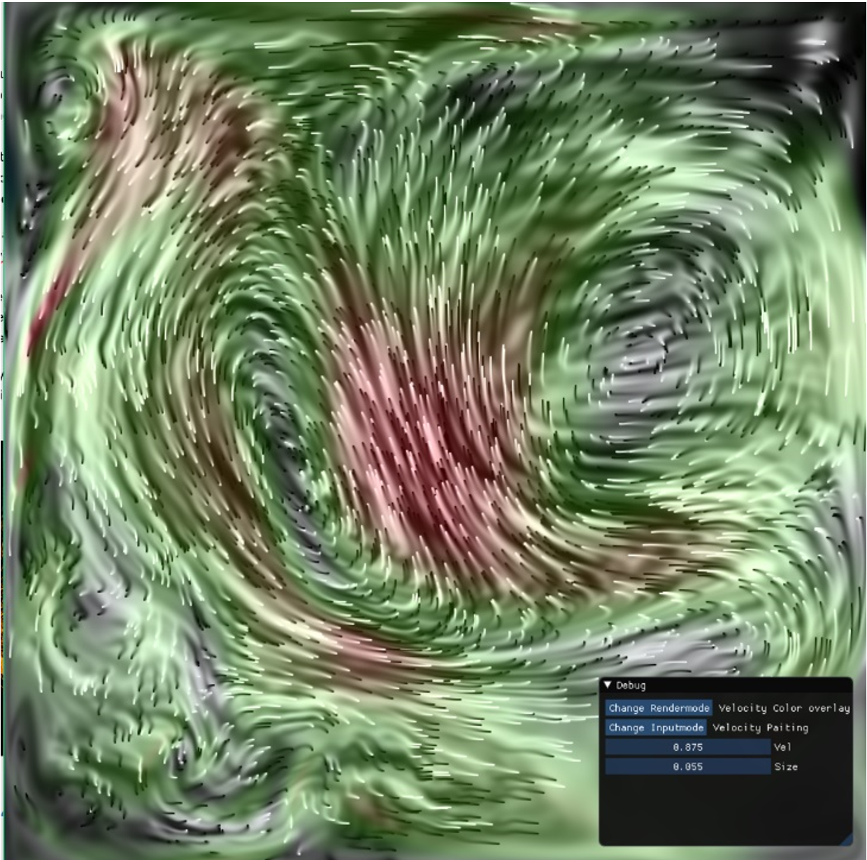
The following video shows some different ways of rendering like rendering the pressure or magnitude of the velocity as a color gradient, different isoline displays, and a hybrid method.
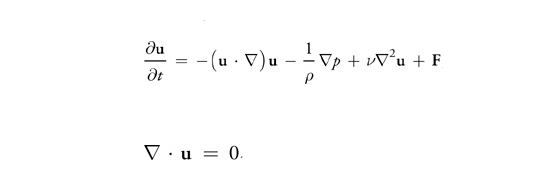
It uses some concepts from vector calculus, there are three different uses for the nabla symbol ∇. The Gradient: ∇p , Divergence: ∇.p and Laplacian: ∇² This set of equations can be split into small pieces: Advection, pressure, vicious diffusion and external forces. It solves these small pieces by using multipass rendering and rendertargets. The function for one step in the simulation of the Liquid simulation (GitHub) looks like this:
            void LiquidRenderer::SimulationStep()
            {
              Advection();
              Diffusion();
              Inflow();
              PressureProjection();
              BoundaryProjection();
            }
Each of these functions binds the input and output textures and then makes its draw calls the the gpu. Each value on the texture represents a discretized small region of fluid. There are multiple textures that contain different values such as pressure, velocity and color. The velocity field texture represents a vector field with while the texture for the pressure is a scalar field. The simplest pass is the advection pass which has two texture inputs. The first one is for a scalar or vector field that represents a quantity to be advected, and the second texture is a vector field with the advection velocities. The velocity field advects the pressure, color and itself in seperate draw calls.
(directx11 hlsl) Advection pixel shader
            PS_OUTPUT PS(VS_OUTPUT input) : SV_TARGET{  // Pixel Shader
              PS_OUTPUT output = (PS_OUTPUT)0;
                float2 vel = gAdvectionForceMap.Sample(samLinear, input.texCoord).xy;
              float2 coords = input.texCoord - (vel.xy / gTextureSize * gTimeStep);
              output.color = gAdvectedQuantityMap.Sample(samLinear, coords);
              return output;
            }
The diffusion term is solved with Jos Stam his implicit backward formulation [stam 1999] using the Jacobi iterative relaxation technique. Performance can be improved by using a better iterative technique but is very good as it is now. Improved performance can be used for additional iterations and more iterations result in better convergence towards an accurate solutiton. This results in a flow with more complex swirling. About 80 iterations are used.
(directx11 hlsl) Jacobi pixel shader
            PS_OUTPUT PS(VS_OUTPUT input) : SV_TARGET{
              PS_OUTPUT output = (PS_OUTPUT)0;
                  float4 Top = gVariableMap.Sample(samLinear, input.texCoord + float2(0, gRes));
              float4 Bottom = gVariableMap.Sample(samLinear, input.texCoord - float2(0, gRes));
              float4 Right = gVariableMap.Sample(samLinear, input.texCoord + float2(gRes, 0));
              float4 Left = gVariableMap.Sample(samLinear, input.texCoord - float2(gRes, 0));
                  float4 Center = gConstantMap.Sample(samLinear, input.texCoord);
              output.color = ((Top + Bottom + Right + Left + (gAlpha * Center)) * (gBeta));
              return output;
            }
Computing the pressure projection term is also done through using the Jacobi pixel shader in the code sample above with the divergence of the pressure and the pressure as inputs, This requires another 80 iterations. The result is substracted from the velocity field.
(directx11 hlsl) Divergence pixel shader
            // Pixel Shader
            PS_OUTPUT PS(VS_OUTPUT input) : SV_TARGET{
              PS_OUTPUT output = (PS_OUTPUT)0;
                float4 varTop = gSourceMap.Sample(samLinear, input.texCoord + float2(0, gRes));
              float4 varBottom = gSourceMap.Sample(samLinear, input.texCoord - float2(0, gRes));
              float4 varRight = gSourceMap.Sample(samLinear, input.texCoord + float2(gRes, 0));
              float4 varLeft = gSourceMap.Sample(samLinear, input.texCoord - float2(gRes, 0));
              output.color.r = (1/ (  gRes)) * ((varRight.x - varLeft.x) + (varTop.y - varBottom.y));
              output.color.a = 1;
              return output;
            }
Boundaries are handled by enforcing that all velocities at the boundary are 0. The pressure is set to 1.
(directx11 hlsl) Boundary projection pixel shader
            // Pixel Shader
            PS_OUTPUT PS(VS_OUTPUT input) : SV_TARGET{
              PS_OUTPUT output = (PS_OUTPUT)0;
              float res = 1 / gTextureSize;
              if (input.texCoord.x < res) {
                float2 coord = float2(input.texCoord.x + res, input.texCoord.y);
                output.color.x = gIsPressure * gDiffuseMap.Sample(samLinear, coord).x;
                output.color.a = 1;
                return output;
              }
              if (input.texCoord.x > 1-res) {
                float2 coord = float2(input.texCoord.x - res, input.texCoord.y);
                output.color.x = gIsPressure * gDiffuseMap.Sample(samLinear, coord).x;
                output.color.a = 1;
                return output;
              }
              if (input.texCoord.y < res) {
                float2 coord = float2(input.texCoord.x , input.texCoord.y - res);
                output.color.y = gIsPressure * gDiffuseMap.Sample(samLinear, coord).y;
                output.color.a = 1;
                return output;
              }
              if (input.texCoord.y > 1 - res) {
                float2 coord = float2(input.texCoord.x , input.texCoord.y - res);
                output.color.y = gIsPressure * gDiffuseMap.Sample(samLinear, coord).y;
                output.color.a = 1;
                return output;
              }
              if (gBoundaryMap.Sample(samLinear, input.texCoord).r > 0.99)
              {
                output.color.a = 1;
                float2 coord = float2(input.texCoord.x + res, input.texCoord.y);
                float s = gBoundaryMap.Sample(samLinear, coord).x;
                if (s < 0.01)
                {
                  output.color.x = gIsPressure * gDiffuseMap.Sample(samLinear, coord).x;
                  return output;
                }
                coord = float2(input.texCoord.x - res, input.texCoord.y);
                s = gBoundaryMap.Sample(samLinear, coord).x;
                if (s < 0.01)
                {
                  output.color.x = gIsPressure * gDiffuseMap.Sample(samLinear, coord).x;
                  return output;
                }
                coord = float2(input.texCoord.x, input.texCoord.y + res);
                s = gBoundaryMap.Sample(samLinear, coord).x;
                if (s < 0.01)
                {
                  output.color.y = gIsPressure * gDiffuseMap.Sample(samLinear, coord).y;
                  return output;
                }
                coord = float2(input.texCoord.x, input.texCoord.y - res);
                s = gBoundaryMap.Sample(samLinear, coord).x;
                if (s < 0.01)
                {
                  output.color.y = gIsPressure * gDiffuseMap.Sample(samLinear, coord).y;
                  return output;
                }
              }
            }
There are many different textures that are used, the ones that are essential to the simulation are the textures that contain the velocity and pressure fields. Additionaly, there is a texture for the color value of each blob of fluid, one to allow users to add fixed boundaries and two to allow for color and velocity inflows. Besides rendering the color texture there are many different ways of visualizing the simulation. Gradient rendering uses a cubic pulse function to create a gradient color for different magnitudes of the velocity.
(directx11 hlsl) Gradient rednering pixel shader
            float cubicPulse(float center, float width, float x)
            {
              x = abs(x - center);
              if (x>width) return 0.0;
              x /= width;
              return 1.0 - x * x*(3.0 - 2.0*x);
            }
            //--------------------------------------------------------------------------------------
            // Pixel Shader
            //--------------------------------------------------------------------------------------
            float4 PS(VS_OUTPUT input) : SV_TARGET{


              float2 Velocity = gAdvectionMap.Sample(samLinear, input.texCoord);
              float vel = sqrt(pow(Velocity.x,2) + pow(Velocity.y,2)) ;
              float4 color = float4(0, 0, 0, 1);
              float t = 1;  //treshhold

              if (vel < 0.00001) return float4(0,0,0,1);
              t = 1;
              color.b += (0.20*cubicPulse(t / 16, t*0.065, vel));
              color.b += (0.15*cubicPulse(t / 8, t*0.125, vel));
              color.g += (0.10*cubicPulse(t / 8, t*0.125, vel));
              color.g +=(0.3*cubicPulse(t/4, t*0.25, vel));
              color.r += (0.7*cubicPulse(t * 2, t * 2, vel));
              color.g += (0.7*cubicPulse(t * 1, t*1, vel));
              color.r += (0.8*cubicPulse(t * 1, t * 1, vel));
              float res = 1024;
              color.b += (0.35*cubicPulse(res * t / 16, res * t*0.065, vel));
              color.g += (0.3*cubicPulse(res * t / 4, res *  t*0.25, vel));
              color.r += (0.7*cubicPulse(res * t * 2, res * t * 2, vel));
              color.g += (0.7*cubicPulse(res * t * 1, res * t * 1, vel));
              color.r += (0.8*cubicPulse(res * t * 1, res * t * 1, vel));

              return float4(color.xyz, 1);

            }